Rollin’ Trees, yo

They are powerful beyond common recognition. Oxygen, life, shelter, food, beauty, computational efficiency, and more are provided by trees when we interact with them in the right ways.

This post will get you familiar with trees and their uses in software. Once you understand the tree, you will be ready to use them in the situations for which they are perfectly suited. Good.

A tree is, first and foremost, a data structure adhering to the interface of the abstract data type Tree. A Tree is just an abstract ideal that we all kind of agree upon — hey buddy, let’s call any data structure that has property X, Y, and Z an array, while any data structure with properties A, B, and L should be called a tree.

Why is this important? Because it helps us avoid a common mental mistake, early — that of confusing the abstract data type Tree with a particular concrete implementation of that abstraction. Can you implement the basic properties of ‘Treehood’ in more than one way? If you answered yes, you are ready to continue. If not, please read about the differences between a concrete entity and an abstraction.

A tree, like all data structures, holds data and has certain data-access rules. Like all data structures, a tree will have tradeoffs related to lookup, insertion, removal, and similar operations. So, here are the real questions:

The tree is often called a ‘node-based data structure,’ like a linked-list or graph — this is just to say that a tree is composed of nodes, where each node stores a value and reference to zero or more other nodes. The tree is distinguished from the other node-based data structures by the constraint that there is a root node and each other node is an ancestor of the root node. This allows the data structure to simulate a tree-like hierarchy that we are used to conceptualizing in disciplines like taxonomy.

Another interesting feature of the tree structure is that each node of a tree is itself a subtree with its own children nodes, making the tree particularly well-suited for interaction with recursion to solve certain types of problem.

Summary:

1. a tree is composed of nodes
2. a tree has a root node
3. each node has a value of any data type
4. a root node has ancestor nodes stored as a list with no duplicates and without the root node itself
5. all nodes are themselves trees

With that summary in mind, here is a simple tree visualization:

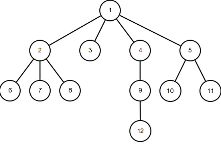
In our case, the top node is the ‘root’ of our tree, storing a value of 1. In this tree, the values being stored at each node are numbers, though this need not be the case. Finally, our root node has 11 ancestors, with only 4 ancestors that are children.

Armed with a firm grasp of the concept of a tree, we can proceed to define the basic structure of a tree implementation.

We are going to create a Tree ‘class,’ from which we can create specific instances of a tree.

Our Tree constructor function takes a single input (the value for the root node). This function will assign the input value to a property on the tree instance, as well as create an empty array to store the children of this root node.

We can now create tree instances right and left (though they will currently lack tree functionality). For example, we don’t have an interface for adding children or checking if a tree contains a child with a given value. But for now, we can at least create trees, like so:

Now that we can make trees, let’s give them a useful interface.

Most agree that a useful tree implementation will at least offer an interface for the following:

1. adding a child node to a tree
2. checking if a child node is in a tree

Those two operations provide a basis for building some cool functionality with your trees, as well as a basis for extension and reuse in other contexts.

Let’s start with adding a node to a tree’s children.

This code is pretty easy to follow:

• we are adding a method called addChild to the Tree .prototype property
• the addChild method takes a single parameter — the value with which to initialize the child tree
• the addChild method pushes a new instance of a Tree initialized with the child value into the children array of the current tree

Next, let’s add a method for checking if a tree contains a node with a target value.

This operation is slightly more complex than addChild because it uses recursion to search through the tree — don’t be alarmed. Let’s break it down.

• we are adding a method called contains to the Tree .prototype property
• the contains method takes two parameters — a target value for which to search the tree and a root node (tree) with which to start the search
• the contains method assigns the root to the root argument passed in or defaults to the current tree
• the contains method sets up a base case to break out of the recursion that we are going to create — if the value at the current root is equal to the target value, we have found the target, i.e., the tree contains the target value
• the contains method iterates through the children of the current root node, recursively invoking the contains method with the same target value to search for, but with a new root tree to search — the child node that is currently being examined in the iteration
• if the recursive call for that child node returns truthy, we know that we have found the target value in that child tree somewhere, so we return true
• finally, if we have searched all of the children trees and not hit our base case, we will return false because we haven’t found the target value anywhere within our tree

This type of recursion through a tree’s children is common. Let’s look at a real-world example of a tree and a function that searches that tree in a similar fashion as our contains method.

The DOM is a tree-like structure. We will ignore the complexities of the DOM, and focus on the properties that allow us to use it as an example of a simple tree. The Document Object Model (DOM) is used in the browser to model an HTML document. The HTML document is represented as a tree of nodes, where each node is an object representation of an HTML element. The root of the tree is the document, which usually has at least two children — head and body.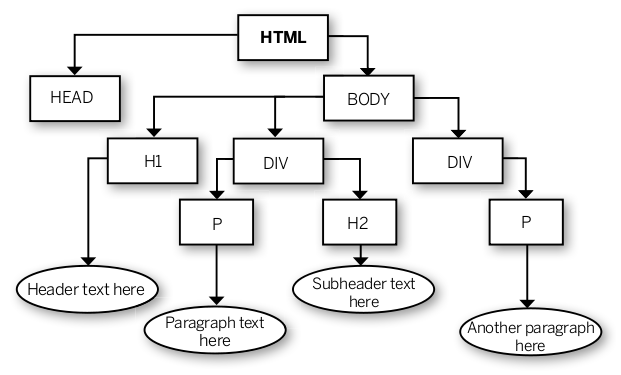

As you can see, head and body are themselves tree-like structures that contain child nodes. Each of those child nodes is also a sub-tree, ad infinitum. Sounds like our simple tree from earlier, right?

If the DOM can be thought of as a tree, then we would assume that some of the DOM API would be similar to the tree interface described above. We would guess that we can search the DOM tree for a given node or a given feature of a node. We would also guess that we can insert child nodes into the DOM tree. In both cases, we would be correct.

I am going to focus on the case of searching the DOM tree, to parallel our contains method from above. There is a JavaScript method called Document.getElementsByClassName(), which searches the document (or any root element) for all of the elements that have a target class name. All elements that have the target classname will be returned from the method call in an array. If no elements are found, the array will be empty. Let’s imagine that we had to write a getElementsByClassName function that mimicks the above functionality.

This looks pretty similiar to the contains method that we wrote above. Here is a line-by-line description:

• line 1: declare global function getElementsByClassName
  • getElementsByClassName takes two parameters — a className to search for and a root node from which to start the search
• line 2: declare nodes variable and initialize to an empty array — will store nodes with matching className
• line 3: assign the node variable to whatever is passed in, or fallback to the document.body node
• line 5: get all of the class names for the current root node by splitting the node.className on whitespace
• line 8: using indexOf, check if the target class name is contained in the list of node’s class names
• line 9: if the target class name was present, push the current node into the matching nodes array
• lines 13 – 16: check children of current node for target class name
  • line 13: iterate the length of the current node’s list of children
  • line 14: for each child, create a variable childResults initialized to the result of invoking getElementsByClassName with the child as the root node from which to start searching
  • line 15: reassign nodes to the current nodes collection concatenated with the childResults from each child
• line 18: return the collection of DOM nodes that have the class name for which the method is searching

By now you should feel comfortable with the simple tree and how it can be used. We aren’t going to stop here though, because the simple tree actually sucks. It is inefficient and rarely used. Let’s discuss the tradeoffs associated with the simple tree.

The simple tree implementation above was for pedagogical purposes, but now let’s examine the costs of this type of tree implementation to see if we can get any clues as to why a simple tree like this is rarely used compared to a more ‘constrained’ tree like a search tree or decision tree.

The time complexity of the addChild operation is constant, so we will ignore addChild for now.

contains is disgusting when it comes to worst-case time complexity. contains iterates through n children, and for each of those iterations, it recurses into checking the children of the current child. This type of recursion nested within iteration is costly — polynomial to exponential.

So, how do we change this costly search operation? How do we make a tree that is optimized to search? Constraint.

The time cost can be greatly reduced by adding constraints to our tree. We could constrain the children. We could also constrain the way that nodes are added to the tree, in order to make it more efficient to search. Let’s turn to the Binary Search Tree as an example of the mentioned constraints.

A common type of tree in computer science is the binary search tree. This tree is similar to the simple tree, but it has a two new constraints:

1. each node can only have 2 children (binary)
2. each node on one side of the tree has one of the possible values of a given binary property, while each node on the other side of the tree has the inverse value for that same given binary property

Let’s keep it simple by using ‘greater than’ and its inverse ‘less than’ as our binary properties.

So, a binary search tree has a root node. That node can have 0 to 2 children. The ‘left’ child will have a value less than our root node, while the ‘right’ child will have a value greater than our root node.

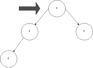
Here is a binary search tree that fulfills those constraints:

 

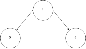
If I asked you to insert a node with a value of 2 into the tree, where would you put it?

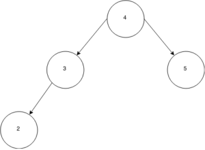
The correct answer is the far left, as the left child of the node with a value of 3. 2 is less than the root value 4, so you look left. 2 is less than the value of 3, so you look left again. You find no more nodes so you insert a node with a value of 2.

You had to check multiple times to make sure that you put the new node in the correct place. This is a constraint on insertion. The binary search tree constrains insertion of new nodes because it is optimized for search — by putting things in a principled order, you can search and retrieve things back out faster than if the tree was unordered. However, the constraints on insertion take time compared to the simple tree that pushed new nodes onto its list of children without checking where to put them. This means that the binary search tree is optimized for read situations and not write situations. So, you would use it in a situation where you need speed for high-frequency search of large data, where you don’t have to write new data to the tree very often (or if you do, it can happen asynchronously in the background with no user waiting on the result). This happens surprisingly often.

Let’s look at the tree in action on search. Let’s say I asked you if your tree contained a node with a value of 2, or if I asked you to return the node with a value of 2 if it exists in your tree?

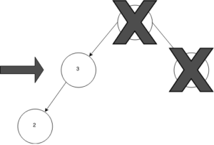
Step 1, check the root of the tree. Is the root value equal to 2? If not, is 2 less than the root’s value?

The root value is 4, so 2 is less than the root node’s value. This means that we need to go look at the left child of the root node, and repeat the process that we just did with the root node. We also get to eliminate the whole right side of the tree because we know that everything on that side is greater than our root node’s value of 4. So, we can ask, is the root’s left child value equal to 2? If not, is 2 less than the root’s left child value?

As you can see, in our case 2 is less than the root’s left child value (3). We can now go down a level in the tree and check the value of the root’s left child’s left child 🙂 Is the value of the left child of the left child of the root equal to 2? If not, is it less than 2?

 

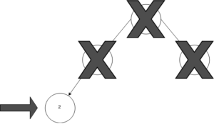
In our case, the value at this node in our tree is equal to our target value of 2, so we can either return true (tree contains value) or return the node itself (node value matches query for node with matching value).

Ok, so that might not seem very impressive, but imagine if your tree (data set) contained millions of nodes. If the tree is balanced like ours, then your first check would possibly cut the query set in half. That is a huge cost cut in time complexity.

Enough theory, you say! Show us the code! Ok, fair enough.

Pretty simple, with heavy dose of recursion. I am going to do a line-by-line, and then discuss the time complexity.

• lines 1 – 5: BinarySearchTree constructor function
  • initializes value property to passed in argument value
  • defaults the left and right child properties to null
• lines 7 – 30: BinarySearchTree insert instance method
  • lines 9 – 11: throws error if you try to insert a duplicate value into the tree
  • line 14: checks if the value to insert is less than the root value
  • line 15: checks if the left child of the root is empty
  • line 16: if empty, inserts a new BinarySearchTree with the passed in argument value
  • line 18: if the left child has a value, try to insert the passed in argument value into the left child
  • lines 23 – 29: run the inverse of lines 9 – 11 for the other side of the tree if the passed in argument value was greater than the root’s value
• lines 32 – 50: BinarySearchTree contains instance method
  • lines 34 – 36: return true if your root value is equal to the target value
    • this is the base case
  • lines 38 – 41: if the value at the root is less than the target value, then you want to check the right side of the subtree
    • if the right child of the root isn’t empty, you want to recurse down that side of the tree to see if it contains the target value
  • lines 43 – 46: if the value at the root is greater than the target value, then you want to check the left side of the subtree
    • if the left child of the root isn’t empty, you want to recurse down that side of the tree to see if it contains the target value
  • line 49: return false if the target value wasn’t found

Compared to the simple tree contains method, the time complexity of the binary search tree contains method is beautiful. All of the comparisons are done in constant time and the recursion is the only linear operation. So, at worst, this search method is linear, compared to the exponential time complexity of the simple tree.

Now that we have built the foundations of the tree and binary search tree, let’s finish this post by examining a very popular use of a special type of tree — the decision tree.

A decision tree is a tree where each node value is dependent on a decision made at a parent node. Sounds abstract, but it is actually pretty intuitive. The tree branches are ‘decision sequences,’ i.e., paths which the decision could take. The key to understanding the decision tree is grasping the idea that each node represents a possible system state. And, each possible system state is determined by its parent’s state.

For example, I am confronted with some choices — dinner or dessert?

If I choose dinner, I am confronted with a new decision point — chicken or steak?

If I choose chicken, I am confronted with a new decision point — fried chicken or chicken marsala?

This could continue as long as we want. Each of the decisions was dependent on the first choice between dinner or dessert. If I had chosen ‘dessert,’ the resulting choices to choose between would have been different than what was offered based on my original decision of ‘dinner.’

We can visualize this example with a decision tree:

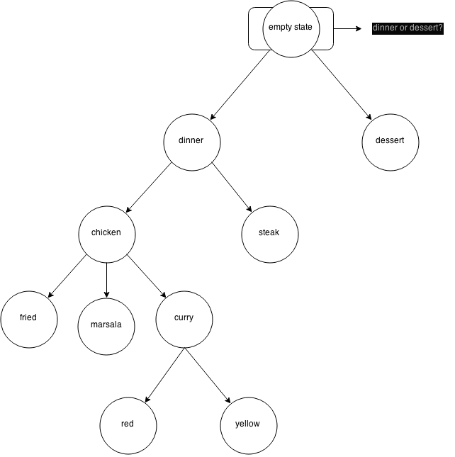
The decision tree will usually contain n * r + 1 nodes, where n is the number or possible choices at each decision point and r is the number of decision points. So, if you have to choose between dinner and dessert, and you only have to make that decision once, then your decision tree would have 3 nodes — one node for each choice (2 nodes total) multiplied by one (number of times you need to make the decision), plus 1.

Humans use this type of ‘branched’ reasoning all the time — don’t let all of the new terminology convince you that a decision tree is anything other than a representation of our standard ‘decision-making’ process.

Look at the tree while imagining that you are sitting in a restaurant with a menu in front of you. The first decision point that you reach is a choice between ordering dinner or dessert (not both, we are strict).

Let’s assume that you want to eat dinner. You will move down a level in the tree to the ‘dinner’ node. Your mind will now prompt you to make another decision — should you order chicken or steak for dinner?

For some reason, you don’t eat red meat, so you decide that you want to have chicken for dinner. Move your focus down to the ‘chicken’ node, and now choose between fried chicken, chicken marsala, or a curry chicken. You love curries, so you move down another node to choose between red and yellow curry.

Once you have made all of the decisions necessary to answer the original question — what you are going to order — you can package up that information into an answer and give it to the server.

But, what is ‘that information’ that you need to package up, and where do you get it?

This is why decision trees are beautiful — your order decision is actually contained within the tree, defined by the sequence of decisions made while traversing the tree. The path that you took is actually your order! You can think of your order as dinner -> chicken -> curry -> yellow, i.e., the values at each of the nodes that were chosen.

Pretty cool, eh?

In reality, our decision-making might require us to go up and down the tree, as well as across the tree, before we can decide on the best final path that we want to take. When we need to do this in our programs, we can harness the properties of the decision tree and use recursion to crawl all over the tree.

You can solve many (software) problems by using a combination of recursion and a decision tree — so, let’s see an example!

At first, I was going to show you my solution to the n-queens problem in order to demonstrate the use of a decision tree, but then I realized how stupid that would be from a pedagogical perspective, due to the complexity of n-queens. I will save n-queens for a separate post. Instead, we are going to use a common toy interview problem based on the rock-paper-scissors (row-sham-bo) game, which isn’t novel but manifests some lessons about using decision trees for system-state analysis.

Prompt: generate an array of all possible throws a single player could throw for n rounds

Constraints of the problem:

• single player
• n rounds
• 3 possible throws — rock, paper, or scissors
• return an array of arrays
  • each internal array is a ‘solution’ — a list of n throws
  • outer array must contain all possible solutions

We can think about this problem as another interaction with a decision tree. We start with an empty state ([]), and then we fill that state with all possible permutations of n throws. We can get an exhaustive list of possible permutations by doing a depth-first-search of a decision tree. Each node represents either a ‘rock’, ‘paper’, or ‘scissor’ throw. We crawl the tree up and down, and each time we get to the end of a branch, we know that we have found a valid solution.

Here is the code, which I will explain below.

We are using a common pattern when working with trees, where we use a recursive subroutine within our solver function.

We start by taking a number of rounds as input — rounds is the number of times the single player makes a throw in a valid solution.

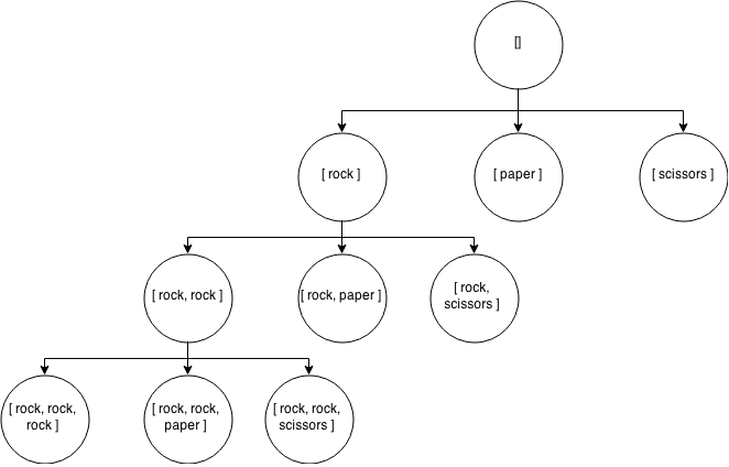
If you look at the tree visualization above, you will see that we start by pushing a ‘rock’ throw into the thrown array. Before we go any further across the tree, we go down the tree with recursion. This happens on line 16, where we recurse with 1 less round of throws.

The recursive call will now push another rock into the array, so we have [ rock, rock ] in our thrown array. Another recursive call will push ‘rock’ into our thrown array one more time, so that we have [ rock, rock, rock ] in our array.

Assuming that we only want our player to throw 3 times (rounds), we will then recurse a final time, passing 0 into our subroutine.

This time, when we enter the recursive call, our base case triggers — we have 0 rounds left to throw, so we know that we have found a valid solution. We have a solution with [ rock, rock, rock ] — we want to push a copy of that solution into our outcomes array in the closure scope. We need to push a copy of the thrown array, because we are going to go back up the tree one level and then find another solution based on that current decision constraint (i.e, [ rock, rock, paper/scissors ]).

This pattern of going down, then up and across, then down, then up and across, etc., will continue n times down, n times up, and plays.length times across. This pattern of movement through the tree is caused by looping across the possible plays, and recursing down n times for each play. Finally, once all of the possible states have been examined through a mixture of iteration and recursion, we know that we have all of our possible outcomes or solutions, so we just return that array of solution arrays.

Hopefully this relatively contrived example shows the value of a decision tree for system-state analysis and sequence analysis.

1. trees are cool
2. trees are node-based data structures
   • each node stores a value and a reference to zero or more children nodes
   • a tree has a root node of which all the other nodes in the tree are ancestors
   • every node is itself a tree, composed of subtrees
3. you can constrain trees to do what you want
   • number of children constraints: binary trees are the most common (each node can only have two children)
   • insertion of data constraints: search trees are the most common (insert data based on a pattern to optimize search and retrieval)
   • type or value of children constraints: decision trees are the most common (the type of node or value at a node is constrained by the values of ancestor nodes)
4. use recursion and smart base cases when working with trees

Save your software, plant a tree.